Three months of “Cumbre Vieja” – analysis of consequences of volcano eruption

Andrzej Mazur
Institute of Meteorology and Water Management – National Research Institute, Poland
Corresponding author’s e-mail: andrzej.mazur@imgw.pl

Keywords: Volcano eruption, atmospheric dispersion, Eulerian model, lagged-ensemble
Abstract

The work describes the methodology and results of analysis for the consequences assessment of eruption from Cumbre Vieja volcano in Canary Islands. The preliminary analysis of dispersion of emitted pollutants was performed using Lagrangian trajectories model. To estimate long-term outcomes of eruption in terms of deposition and concentration of eruption products the Eulerian model of air dispersion was used. The model used data from Global Forecasting System meteorological model launched at the NCEP–NOAA centre. The average concentration and deposition of sulfur compounds as well as the probability and time of the pollution cloud reaching all European capitals were examined. In 90 days a cloud of pollutants (SO₂, volcanic ashes) spread over the northern hemisphere. Pollution reached Africa, North Sea and Europe. With an average emission of 15,000 tons of SO₂/day, maximum calculated deposition to the Earth’s surface reached 0.8g/m², while overall deposition – 35 kilotons in the domain area.

Introduction

The volcano called Cumbre Vieja has a ridge that runs in a north-south direction and covers the southern part of the island La Palma in Canary Islands, with its top and sides riddled with many craters. The last eruption – lava, ashes, sulfur and carbon dioxide – was underway continuously from 19.09.2021 up to 21.12.2021. Initially, the estimated sulfur dioxide emission was around 25 kilotons per day. During the eruption period, the average intensity of the eruption decreased from a maximum value of 36 to 10 kilotons SO₂. The products of the eruption, especially SO₂, CO₂ and volcanic ashes, were constantly transported in the air over northern Africa and Europe. The aim of the study was to analyze and assess environmental consequences of the eruption. By “environmental” one should understand the magnitude and extent of the dispersion of pollutants.

Two basic factors influence the quality of the operational assessment and analysis of an emission incident. The first is reliable quantitative data on emissions, including effective emission height, its vertical profile and mass flow of pollutant (contamination) released. The second is reliable meteorological data that would allow for description of the atmospheric dispersion of pollutants. Considering the amount of emission in any case of a release of hazardous substances obtaining quantitative information is usually very difficult and involves a significant risk. In this study the best emission data that can be obtained comes from satellite measurements. Emission data for this simulation came from (NASA 2021). Weekly variability of emitted SO₂ is presented in Table 1.

Table 1. Variability of weekly emission of SO₂ during eruption of Cumbre Vieja, from 19.09.2021 to 21.12.2021.

Day	SO2 emission, kilotons
09-19-2021	28.3
09-22-2021	36.0
09-29-2021	11.5
10-06-2021	7.5
10-13-2021	17.3
10-20-2021	21.6
10-27-2021	23.2
11-03-2021	25.0
11-10-2021	5.0
11-17-2021	5.5
11-24-2021	7.0
12-01-2021	5.5
12-08-2021	1.8
12-15-2021	0.8

 

Sources:

• NASA Atmospheric Chemistry and Dynamics Laboratory Global Sulfur Dioxide Monitoring, webpage https://so2.gsfc.nasa.gov/volcano_past.html
• own elaboration

In turn, the meteorological data necessary for modeling the atmospheric dispersion of sulfur compounds come from the GFS (Global Forecasting System) model, launched by the NCEP-NOAA (National Centers for Environmental Prediction – National Oceanic and Atmospheric Administration). During the research, a time subset of the necessary data and a spatial sub-region adapted to the domain of the dispersion model were selected. The possibility of online selection is available using dedicated server (NOMADS 2021). For the simulation 120-hour sequences (with the time interval of 1 hour and with a spatial resolution of 0.25 degree) of meteorological fields forecasts necessary for the work of dispersion model were selected and recalculated to the model domain. The dispersion model equations were formulated in rotated latitude-longitude geographical coordinates and terrain-following height coordinate (see Schaettler & Blahak 2013 and Mazur et al. 2014, respectively). The domain of the dispersion model is shown in Figure 1. Overall, the domain size was 295 x 245 grids of 28x28km.

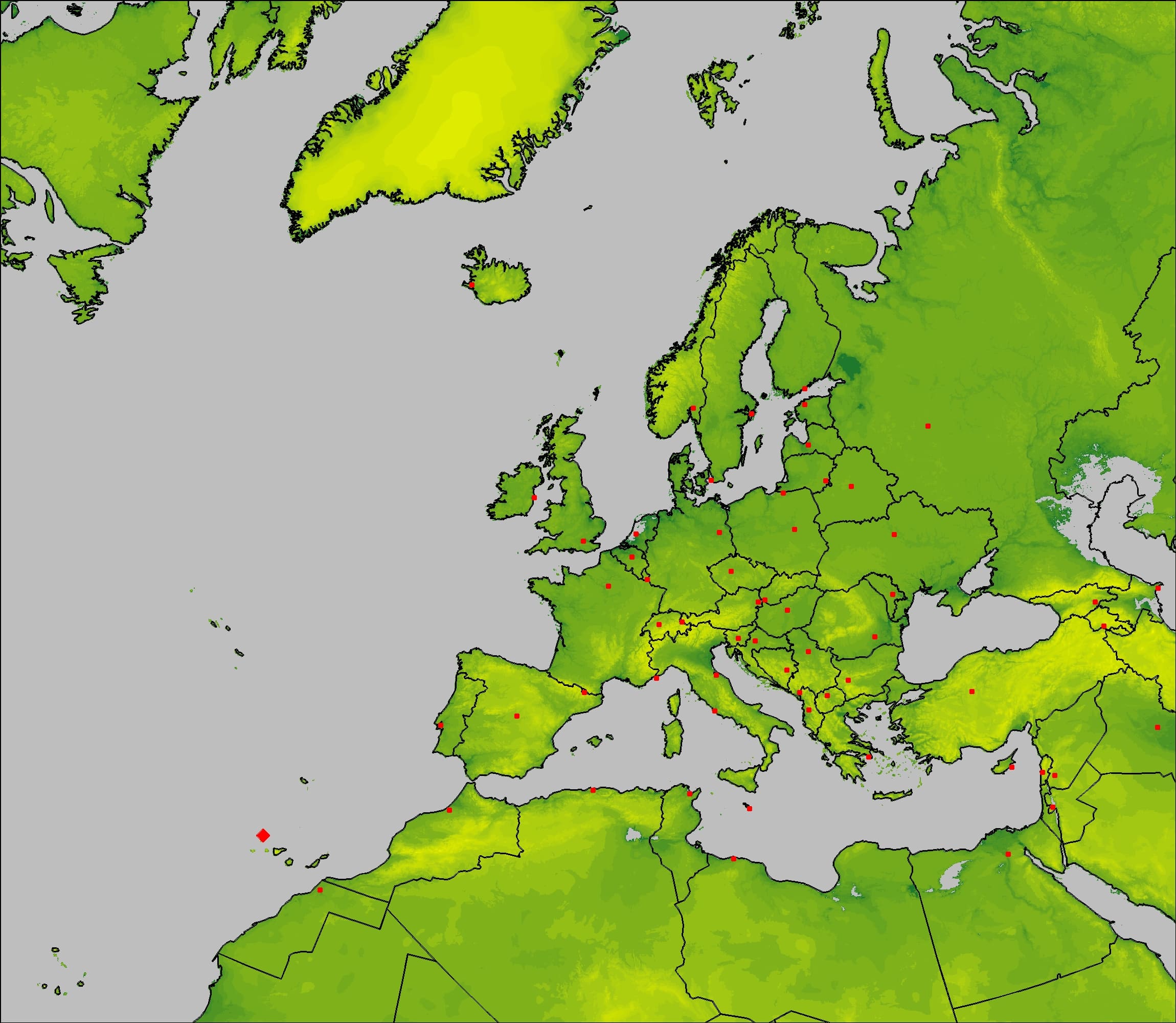
Figure 1. Domain of atmospheric dispersion model – grid size 295 x 245, resolution 28km, rotated latitude-longitude coordinates. Big red diamond marks location of the volcano. Red dots represent of capital cities located within the domain.

Methods

Meteorological data

The quality of the dispersion simulation results depends inter alia on the reliable meteorological data. These, in turn, can be “improved” by applying the lagged-ensemble technique (Bouallegue et al. 2013, DelSole et al. 2017). Basically, lagged-ensemble is a set of forecasts from the same model initiated and launched at different times, but giving forecasts for the same period. For example, if a time horizon for single forecast is five days and forecasts are computed every six hours, there is a time window during which results of every forecast model run are common. The diagram of this technique is shown in Figure 2. Using weather forecasts for sufficiently long period one can obtain a set of twenty members ensemble via moving the time window as illustrated in Fig. 2. Most of authors (Chen et al. 2013, Lu et al. 2007, Yuan et al. 2009) stated that the use of the lagged ensemble method improved forecasts. Taking advantage of the fact that meteorological data from the NOMADS server were available daily for seven days back, this work used this scheme for the entire considered period.

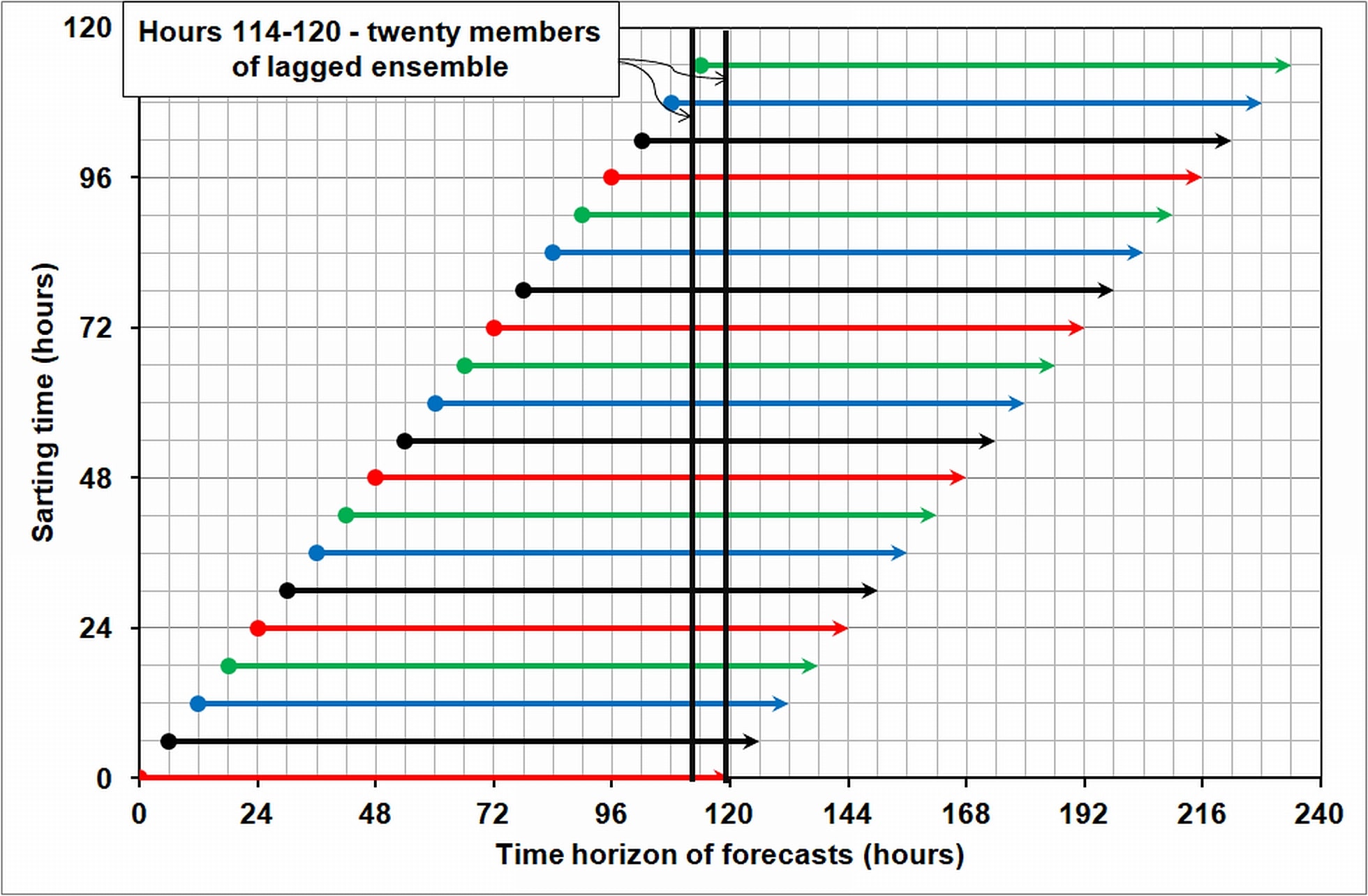
Figure 2. The idea of a lagged ensemble – an example. X-axis – time horizon of forecasts for consecutive runs of meteorological model. Y-axis – starting time of consecutive model runs. The space between two vertical black lines depicts 6-hours-long time period common for all 20 runs.

Basic meteorological data used in this study were the 3D-wind fields, the precipitation amount and other values necessary to determine coefficient of turbulent diffusion and dry deposition velocity (e.g. Mazur et al. 2014).

Chemical transformations

To simplify the calculations it was assumed that the only chemical transformation in case of sulfur compounds was the transformation of sulfur dioxide (SO₂) into sulfate (SO₄^-2), according to the abridged description as stated by (Mazur 2016, see also Kryza et al. 2010). The type of sulfur compound determines the dry deposition velocity and washout ratio, respectively (Mazur 2008). The conversion rate from sulfur dioxide to sulfate aerosol was set to a constant rate of 1% per hour, following (Businger et al. 2015). A direct result of the conversion was an increase of washout ratio and decrease of dry deposition velocity, to be taken into account in calculations.

Trajectory analysis – introduction

The idea of a trajectory analysis based on the work of (Nordlund et al. 1998, see also Mazur 2019). Processed wind fields were used to calculate 10-day trajectories from the release point at all standard pressure levels that can be assumed as an average effective emission levels. One trajectory was released every ten minutes of the entire period of study. The time step between successive points on every trajectory was five minutes to ensure the stability condition (so-called CFL – Courant-Friedrichs-Lewy condition, see e.g. Lax 2013) stating that the distance between two successive points is smaller than the grid size (28 km). Almost two hundred thousand trajectories were calculated during the period of interest. The methodology of calculating the trajectory was identical to that in (Bartnicki et al. 2010) but extended to a three-dimensional problem, such as in (Pongkiatkul & Kim Oanh 2007, Draxler 2007).

Trajectory analysis – probability maps and Estimated Time of Arrival (ETA).

Every released trajectory passed of course the grid square including the location of the volcano. Thus, the calculated probability for this grid was equal to one – the maximum value for the entire domain. The probability of arrival to any other grid is equal to number of trajectories passing through this grid divided by a total number of all trajectories. Computed probability of arrival depends on the length of the trajectories – in general, the probability of arrival slightly increases with the length of the trajectory. That is why, to maintain consistency of selected meteorological conditions, full 10-day trajectories were used in the computations.

Eulerian model – introduction

Atmospheric dispersion of pollutants in an Eulerian approach may be expressed with a system of partial differential equations describing advection, diffusion, emissions and removal, that can be solved independently in every horizontal and vertical direction (see Mazur 2008, also De Visscher 2014). First, horizontal advection part is resolved using a numerical Area Preserving Flux algorithm developed by (Bott 1989). This time-implicit, positive defined and mass-conservative algorithm is applied horizontal directions at every time step, while diffusion term was solved with semi-implicit Crank-Nicholson method (Mazur 2008). Hence, the model in general meets the criteria of the first-generation Eulerian Grid Model (Juda-Rezler 2010).

Results and Discussion.

Trajectory analysis.

A map with the probability of trajectory arrival to every grid of the domain is shown in Figure 3. This map answered the following question: ”what was the probability that the pollution cloud as a result of the eruption would arrive to certain locations in Europe?”

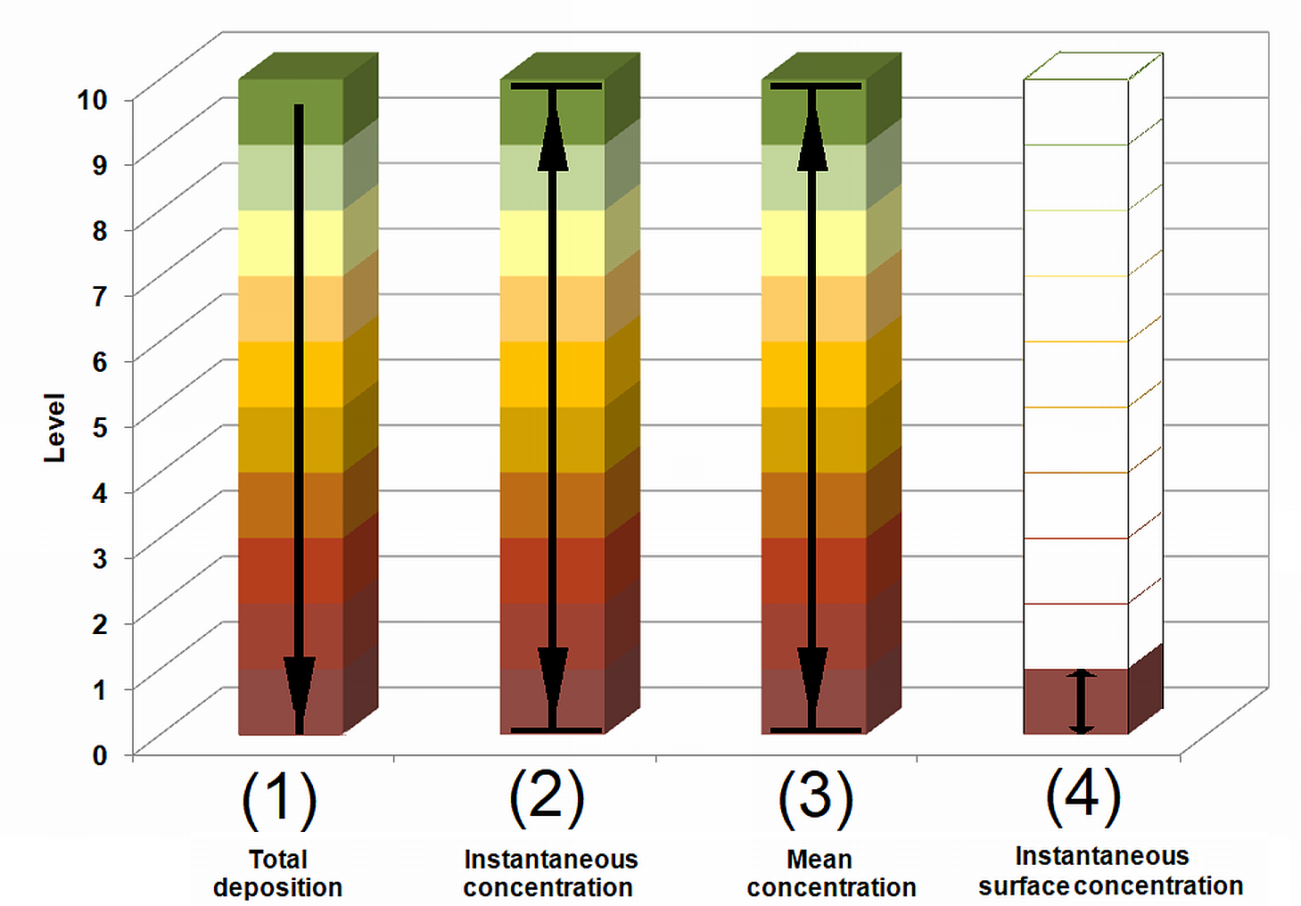
Figure 3. Schematic representation of variables of consideration. Justify to right: (1) total deposition, (2) instantaneous concentration, (3) mean concentration, (4) instantaneous surface concentration. Further explanations in text.

Of course, since the volcano is located close to the continent, the probability is generally quite similar for the entire territory of Europe. However, specific locations may significantly differ in this respect. Thus the next question to be answered is: “how fast the contamination cloud would reach specific locations in Europe?” To answer this, mean travel time was calculated in three steps. Firstly the number of trajectory points starting in Cumbre Vieja and reaching the specified grid was calculated. For each trajectory counting was started from the second point omitting the exact starting location (first point). Then the number of points counted was multiplied by the trajectory time step (five minutes) to calculate the total travel time. Calculated travel times were stored for every grid, making it possible to calculate the spatial distribution of the mean ETA for the entire domain. However, it should be remembered that due to the large area of the domain and the relatively short research time, the trajectories did not reach all points. Space distribution of the mean ETA to each grid of the area of interest is shown in Figure 4.

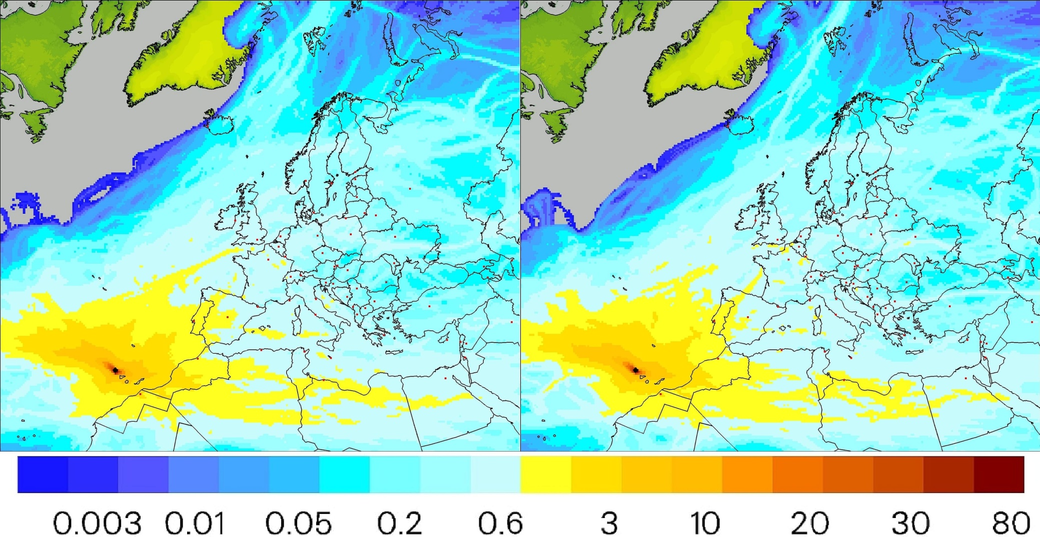
Figure 4. Maps of probability [%] of trajectory arrival to every grid square of the model domain, calculated on the basis of trajectory analysis (19.02.2021–21.12.2021). Justify – results of deterministic approach. Right – results of lagged-ensemble approach.

Eulerian model.

The entire period of the volcanic eruption was examined in the second part of the study using the Eulerian dispersion model. Contrary to the trajectory method it was assumed that the emission took place simultaneously on many levels of the model, in accordance with the assumed profile as in Figure 5. This profile assumption was due to the fact that the total emission from most volcanic eruptions (especially hot steam and sulfur dioxide emissions) consists of hot and light highly buoyant particles close to the source tending to move upwards rather than downwards (Eckhardt et al. 2008, Carboni et al. 2016).

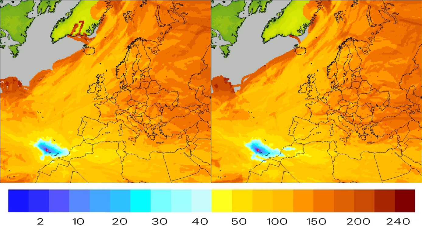
Figure 5. Map of the mean arrival time [hours] to every grid square in the model domain (19.02.2021–21.12.2021). Transparent areas (with no color assigned) pertain to grids that none of ten-day trajectories ever reached during considered period. Justify – results of deterministic approach. Right – results of lagged-ensemble approach.

In this work four variables were analyzed as the results of the Eulerian model (Figure 6). First, it should be noted that both deterministic and lagged-ensemble outcomes were analyzed according to the proposed methodology. The first analyzed field was total deposition (Figure 6, chart 1). This quantity determines the overall contamination flux of sulfur to the soil as a result of scavenging and/or settlement, i.e. wet or dry deposition, respectively.

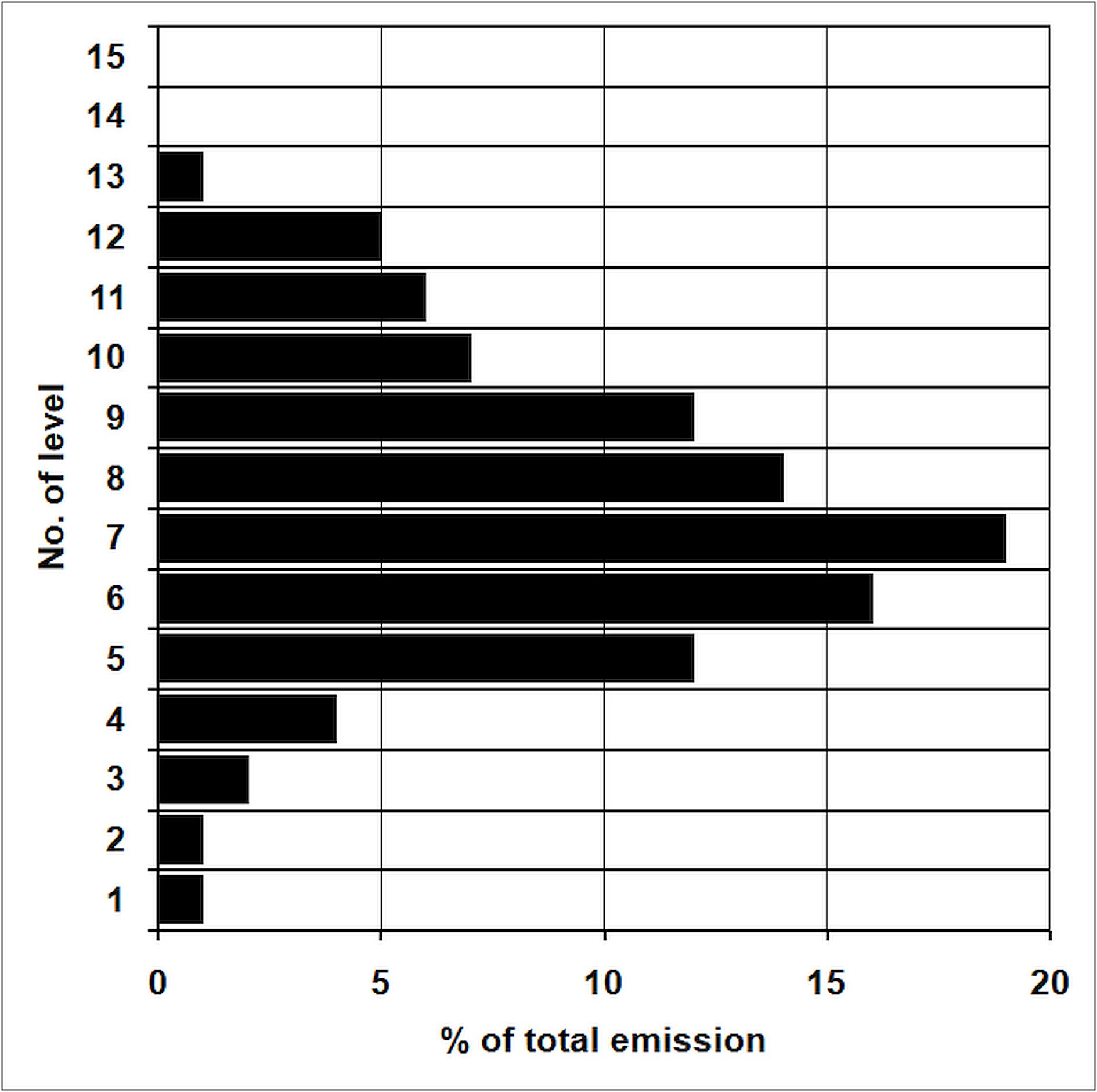
Figure 6. Emission profile – amount of emission vs. emission height. Y axis – no. of model level (1 to 15); X axis – relative (percentage) amount of emission at selected level (total emission at all levels equals 100%).

In the Figure 7 the distribution of deposition due to emission from Cumbre Vieja and atmospheric transport of sulfur dioxide for all the considered period is presented. Values of deposition was presented as milligrams per square meter in a single model grid. As per the above note, justify chart shows results of deterministic approach and right – results of lagged-ensemble approach.

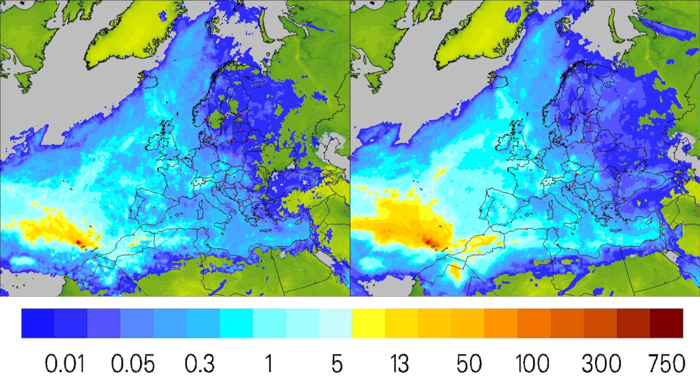
Figure 7. Distribution of total deposition [mg/m²] due to emission from Cumbre Vieja and atmospheric transport of sulfur compounds (expressed as SO₂) in the period 19.02.2021–21.12.2021. Justify – results of deterministic approach. Right – results of lagged-ensemble approach.

Another field of study was instantaneous concentration, i.e. the mean value in the vertical column from the ground surface to the top of the model (Figure 6, chart 2). The distribution of instantaneous concentration values (obtained for the last day of simulation, i.e. 21.12.2021), expressed in micrograms per cubic meter in a single model grid is shown in Figure 8.

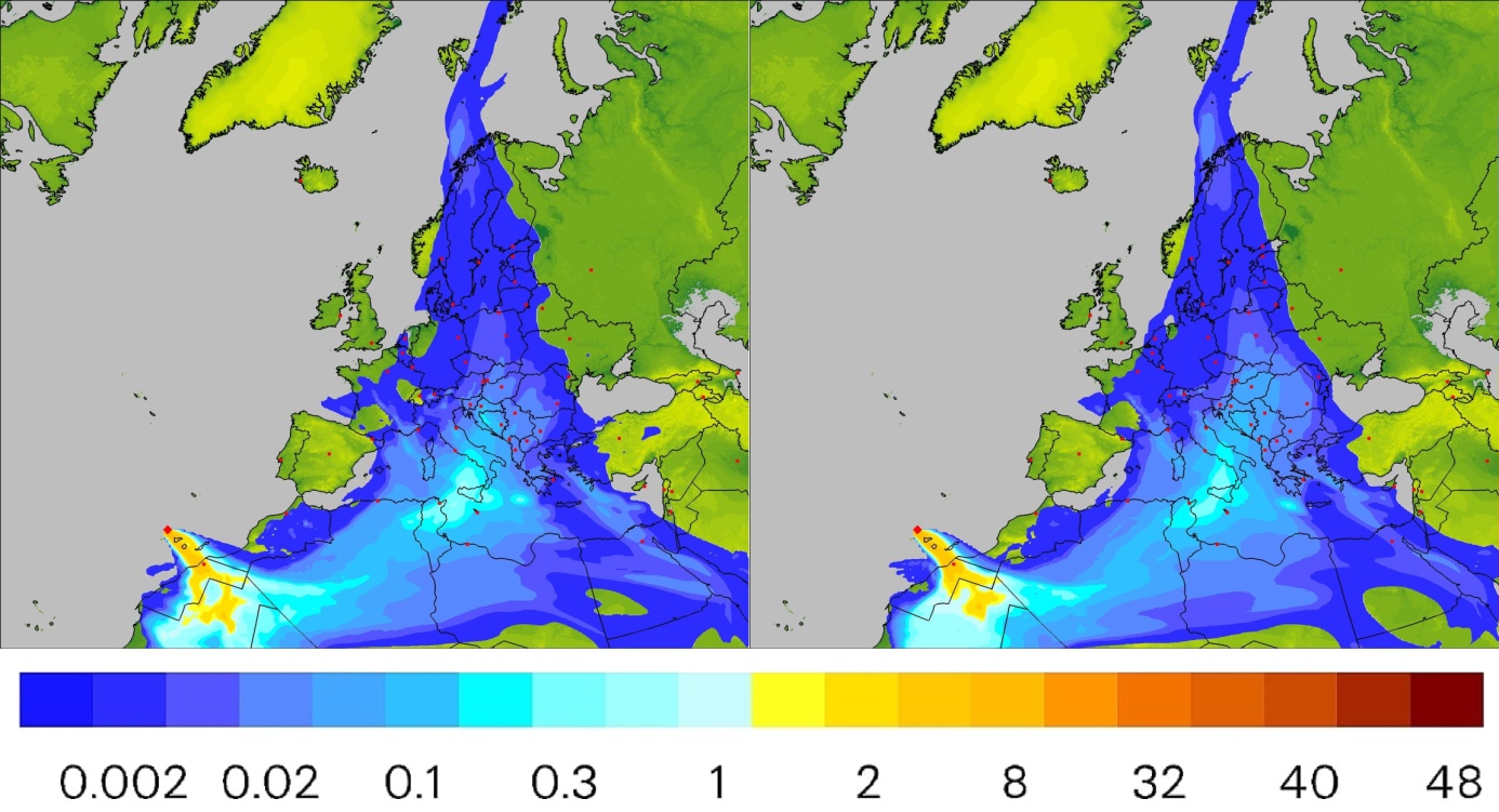
Figure 8. Distribution of mean instantaneous values of concentration [μg/m³] due to emission from Cumbre Vieja and atmospheric transport of sulfur compounds (expressed as SO₂) as calculated for 21.12.2021. Justify – results of deterministic approach. Right – results of lagged-ensemble approach.

The third calculated variable was the average value of concentration in the vertical column from the ground surface to the top of the model (Figure 6, chart 3) over the entire period, i.e. the averaged over the time the above-mentioned instantaneous concentration. The results obtained in the simulation are presented in Figure 9.

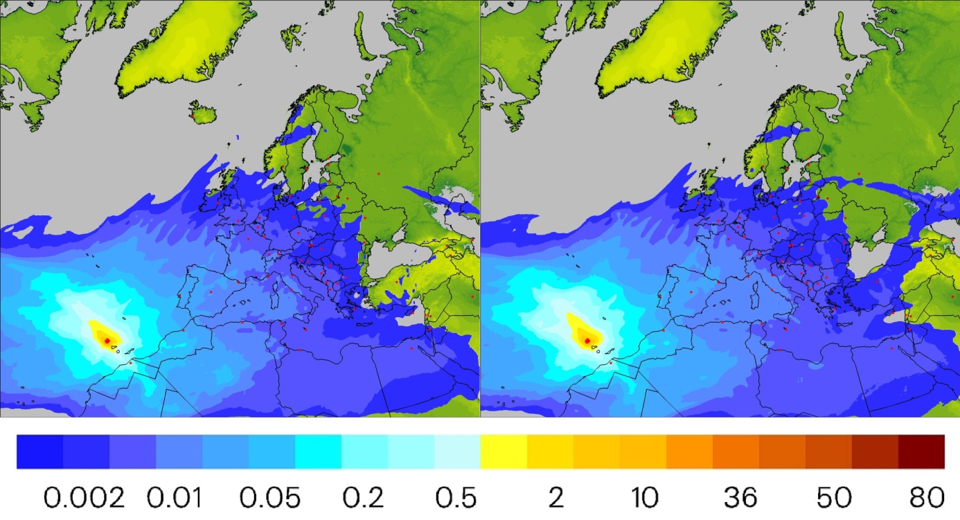
Figure 9. Distribution of overall mean values of concentration [μg/m³] due to emission from Cumbre Vieja and atmospheric transport of sulfur compounds (expressed as SO₂) in the period 19.02.2021–21.12.2021. Justify – results of deterministic approach. Right – results of lagged-ensemble approach.

Finally, the instantaneous value of concentration at the model level closest to the Earth’s surface (Figure 6, chart 4), i.e. time-mean surface concentration is shown in Figure 10.

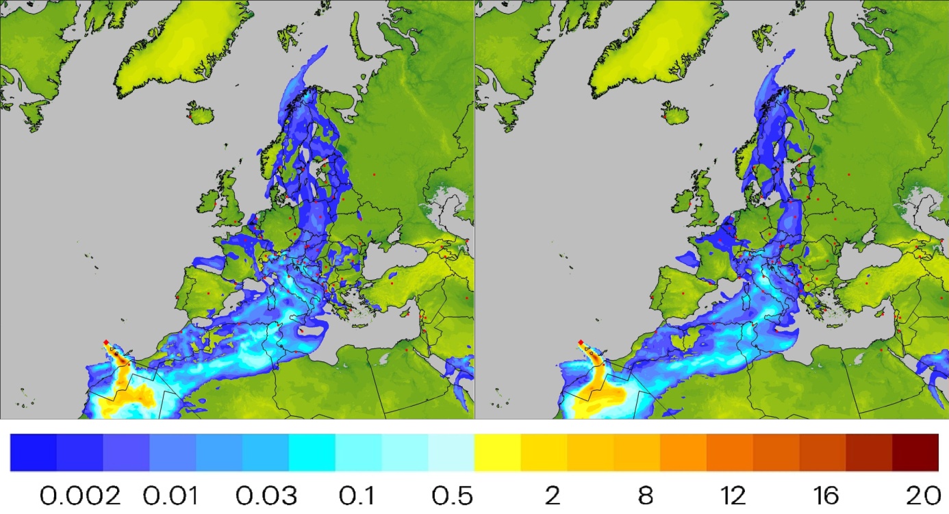
Figure 10. Distribution of instantaneous surface values of concentration [μg/m³] due to emission from Cumbre Vieja and atmospheric transport of sulfur compounds (expressed as SO₂) as calculated for 21.12.2021. Justify – results of deterministic approach. Right – results of lagged-ensemble approach.

From results presented in Figures 7 and 9 it can be concluded that the main direction of sulfur dioxide dispersion was west-northwest (yellow and red colors in the deposition and average concentration distributions presented in these Figures). This is an outcome of the fact that at least in the first period – from about a month to five weeks from the beginning of the eruption – it was the main path of winds controlling the dispersion (advection) of pollution. Subsequently, from the beginning of November, the wind changed so much that the flow from the west to the east-northeast started to dominate. Then, clouds of sulfur compounds much more often reached central Europe, changing the distribution of instantaneous concentration values and surface concentration – as shown in Figures 8 and 10, comparing to the average values (Figures 7 and 9). This conclusion can be confirmed using the results presented in Figures 3 and 4. The spatial distribution of the probability of impact by the pollution cloud was shifted – in accordance with the above argumentation – to the west and north-west direction. In turn, the distribution of estimated time of arrival (ETA) to points in the domain was displaced to east and north-east. It was mainly due to the predominant dispersion directions in the second half of the eruption period and stronger winds during that time.

It should be kept in mind that assuming the average emission of 15 kilotons of SO₂ per day, the calculated deposition maximum reached about 0.8 g/m² (close to the emission point) and the total accumulated deposition to the Earth surface in the domain area was calculated as about 35 kilotons, expressed as SO₂, or around 12000 tons of atomic sulfur. To this amount one should also add the total amount of the pollutant in the air – around 380 kilotons of SO₂. The total figure was about 420 kilotons of sulfur compounds, compared to 1350 kilotons emitted SO₂. The conclusion from these calculation is that about two-thirds of total amount of sulfur compounds justify the computational domain as it can be supposed especially in the first period of the eruption.

The last element examined in the study was the time series of concentration and deposition over selected points (capital cities located within the domain, see Figure 1). In Figure 11a and 11b an example of time courses of instantaneous concentration (μg/m³), surface concentration (μg/m³) and deposition (mg/m²) over Warsaw due to emission from Cumbre Vieja and atmospheric transport of sulfur dioxide in the period 19.09.2021–21.12.2021 in deterministic and in ensemble approach is shown.

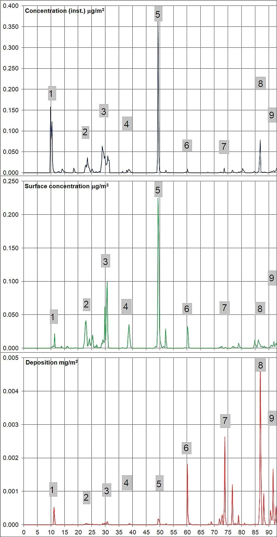
Figure 11a. Top to bottom: time courses of instantaneous: concentration (μg/m³), surface concentration (μg/m³) and deposition (mg/m²) over Warsaw due to emission from Cumbre Vieja and atmospheric transport of sulfur compounds (expressed as SO₂) in the period 19.09.2021–21.12.2021. X-axis – successive days of simulation. Numbers from 1 to 9 mark selected time maxima of deposition and/or concentration. Results of deterministic approach.

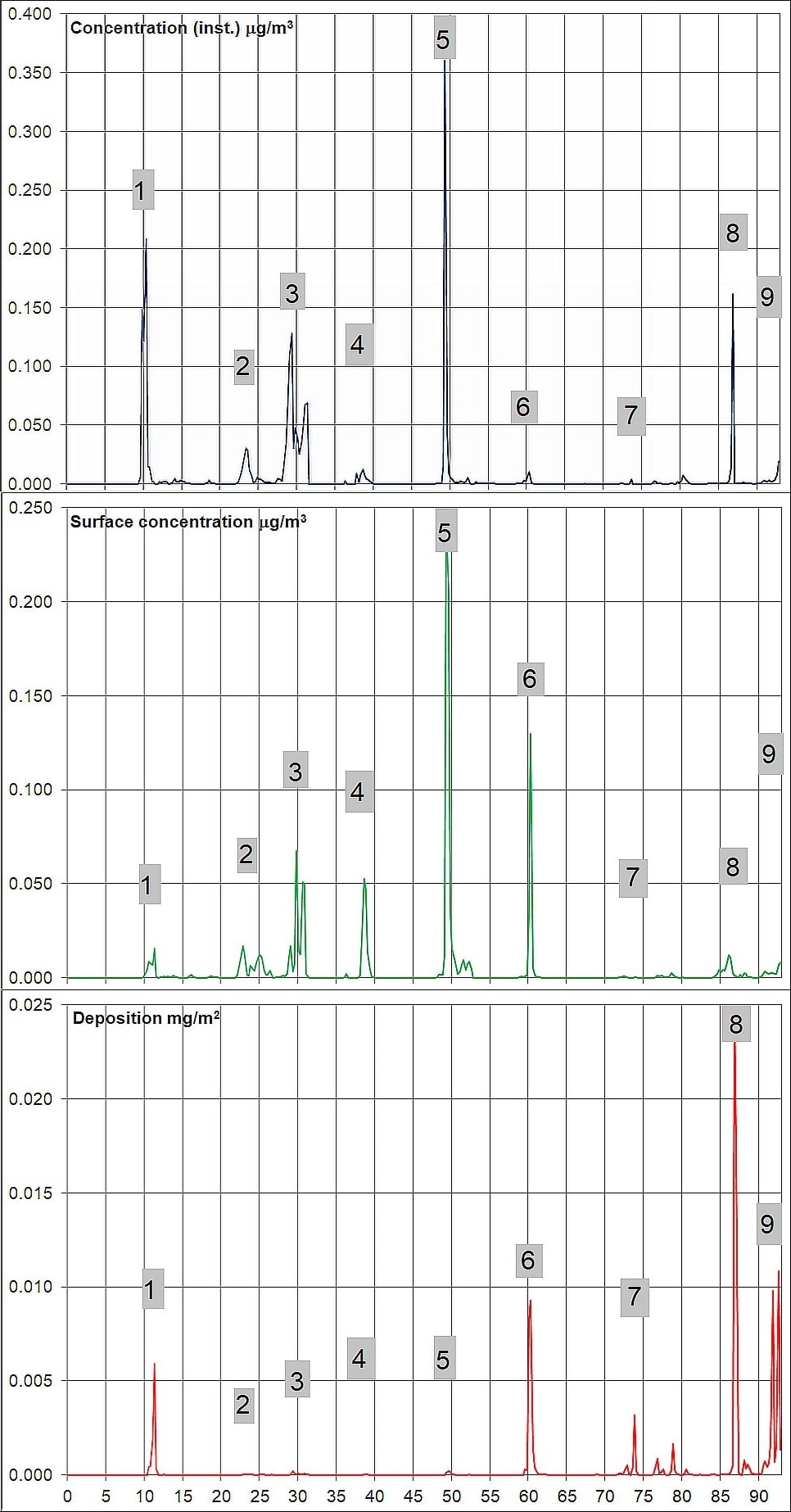
Figure 11b. Top to bottom: time courses of instantaneous: concentration (μg/m³), surface concentration (μg/m³) and deposition (mg/m²) over Warsaw due to emission from Cumbre Vieja and atmospheric transport of sulfur compounds (expressed as SO₂) in the period 19.09.2021–21.12.2021. X-axis – successive days of simulation. Numbers from 1 to 9 mark selected time maxima of deposition and/or concentration. Results of lagged-ensemble approach.

All the dates of maxima shown in the Figure 11 are presented in Table 2. Using the previously described trajectory analysis, it was checked which of trajectories released during the volcanic eruption reached the receptor – Warsaw – on those days and at similar hours.

Table 2. Time maxima of instantaneous concentration, surface concentration and deposition over Warsaw during eruption of Cumbre Vieja, from 19.09.2021 to 21.12.2021.

No. as in Figure 11	Start day/ End day	Hours of trajectory release/arrival (UTC)
		Deterministic approach	Lagged-ensemble approach
1	September 21st September 29th	17:00 22:00	11:00 22:00
2	October 7th October 11th	03:00 21:00	09:00 19:00
3	October 11th October 19th	01:00 09:00	19:00 05:00
4	October 21st October 25th	05:00 08:00	05:00 10:00
5	October 28th November 7th	23:00 06:00	11:00 10:00
6	November 8th November 17th	10:00 19:00	12:00 18:00
7	November 23th December 1st	23:00 17:00	20:00 20:00
8	December 10th December 14th	10:00 17:00	16:00 18:00
9	December 15th December 19th	00:00 21:00	01:00 09:00

Source: own elaboration.

Additionally, to assess the influence of local meteorological conditions, the amount of precipitation as well as local field conditions that affect the amount of dry deposition were determined. Similar results were obtained for both the deterministic and for lagged-ensemble approach. On the basis one can suppose that:

• deposition maximum #1 is due to relatively little rainfall (approx. 0.5 liters/m²) combined with dry deposition from the lowest level (closest to the Earth’s surface).
• deposition maxima #2-5 are only due to dry deposition as a result of no precipitation.
• deposition maximum #6 is the result of washout of a relatively low concentration as a result of rainfall with an intensity of about 2 l/m².
• deposition maxima #7-9 were the result of wet deposition – scavenging from low concentration with intense precipitation, above 5 l/m².

Similar analysis has been prepared for other receptor points.

Conclusions.

The main aim of this research was to answer a question of what were the effects of environmental pollution and the impact of the eruption of the Cumbre Vieja volcano on a regular activity of human population. Despite the emission lasting over 90 days, it seems that these effects were less severe than, for example, in case of the eruption of Eyjafjallajökull volcano in Iceland (April 2010). No micro-particles of silica and volcanic ash were emitted to/detected at cruising altitudes of civil aviation, so there was no need to stop air traffic (“flight bans”). Nevertheless, almost all of Europe was under the contamination cloud, and the average deposition value (expressed as sulfur dioxide) in the domain was around 0.6 mg/m².

The fastest time for a pollution cloud to reach most European capitals was around 20 hours, while the mean – 100 hours or four days.

The following calculation may prove the intensity of the eruption and the scale of the size of the emitted pollutants. In the study (Mazur, 2016) it was shown that the average annual amount of deposition in Poland from emission sources located outside Poland was approximately around 40 mg/m². The SO₂ from the volcano gave an additional contribution of (on average) 1 mg/m² over 90 days, which is 4 mg/m² per year. This corresponds to about 2.5% of the real eruption time, or 10% per year.

It is difficult to talk about a quantitative verification of the results because no direct field measurements (of deposition) were made, and the only current source of information about the actual concentration values were satellite images. Nevertheless, the results achieved with the deterministic and lagged-ensemble approach were similar. The application of the lagged- ensemble approach causes the “smoothing” of spatial distributions – compared to the results achieved in the deterministic approach, the distributions are visually flattened. However, since the use of the lagged-ensemble approach in current calculations uses the most recent and the most up-to-date information and data, it seems logical to use such an approach if it is possible.

Literature

Bartnicki, J., Haakenstad, H. & Benedictow, A. (2010). Atmospheric transport and deposition of radioactive debris to Norway in case of a hypothetical accident in Leningrad Nuclear Power Plant. Met.no report 1/2010. Norwegian Meteorological Institute, Oslo.

Bouallegue, Z.B., Theis, S.E. & Gebhardt, C. (2013). Enhancing COSMO-DE ensemble forecasts by inexpensive techniques. Meteorologische Zeitschrift 22, 1, pp. 49–59. DOI:10.1127/0941-2948/2013/0374

Bott, A. (1989) A positive definite advection scheme obtained by nonlinear renormalization of the advective fluxes. Mon. Wea. Rev. 117, pp. 1006-1015, DOI:10.1175/1520-0493(1989)117<1006:APDASO>2.0.CO;2

Businger, S., Huff, R., Horton, K., Sutton, A.J. & Elias, T. (2015). Observing and forecasting vog dispersion from Kīlauea Volcano, Hawaii. Bull. Amer. Meteor. Soc. 96, pp. 1667-1686. https://doi.org/10.1175/BAMS-D-14-00150.1

Carboni, E., Grainger, R.G., Mather, T.A., Pyle, D.M., Thomas, G.E., Siddans, R., Smith, A.J.A., Dudhia, A., Koukouli, M.E. & Balis, D. (2016). The vertical distribution of volcanic SO₂ plumes measured by IASI. Atmos. Chem. Phys., 16, pp. 4343–4367, DOI:10.5194/acp-16-4343-2016

Chen, M., Wang, W. & Kumar, A. (2013). Lagged ensembles, forecast configuration, and seasonal predictions. Mon. Wea. Rev. 141, no. 10, pp. 3477-3497. DOI:10.1175/MWR-D-12-00184.1

DelSole, T., Trenary, L. & Tippett, M.K. (2017). The Weighted-Average Lagged Ensemble. J. Adv. Model Earth Syst. 9, 7, pp. 2739–2752. DOI: 10.1002/2017MS001128.

Draxler, R.R. (2007). Demonstration of a global modeling methodology to determine the relative importance of local and long-distance sources. Atmos. Env. 41, pp. 776-789, DOI: 10.1016/j.atmosenv.2006.08.052

Eckhardt, S., Prata, A.J., Seibert, P., Stebel, K. & Stohl, A. (2008). Estimation of the vertical profile of sulfur dioxide injection into the atmosphere by a volcanic eruption using satellite column measurements and inverse transport modeling. Atmos. Chem. Phys. 8, pp. 3881–3897, DOI:10.5194/acp-8-3881-2008

Juda-Rezler, K. (2010). New challenges in air quality and climate modeling. Arch. Environ. Prot., 36, 1, pp. 3-28

Kryza, M., Błaś, M., Dore, A.J. & Sobik, M. (2010). Fine-Resolution Modeling of Concentration and Deposition of Nitrogen and Sulphur Compounds for Poland – Application of the FRAME Model. Arch. Environ. Prot., 36, 1, pp. 49-61

Lax, P.D. (2013). Stability of Difference Schemes, in: de Moura, C.A. & Kubrusly C.S. (eds.) The Courant–Friedrichs–Lewy (CFL) Condition 80 Years After Its Discovery. ISBN 978-0-8176-8393-1, DOI 10.1007/978-0-8176-8394-8 Springer New York Heidelberg Dordrecht London

Lu, C., Yuan, H., Schwartz, B.E. & Benjamin, S.G. (2007). Short-range numerical weather prediction using time-lagged ensembles. Weather and Forecasting 22, 3, pp. 580–595. DOI:10.1175/WAF999.1

Mazur, A. (2008) Unified model for atmospheric transport of pollutants over Poland. Doctoral Dissertation. (in Polish) Warsaw, IMGW.

Mazur, A., Bartnicki, J. & Zwoździak, J. (2014). Operational model for atmospheric transport and deposition of air pollution. Ecol. Chem. Eng. – S 21, 3, pp. 385-400, DOI: 10.2478/eces-2014-0028.

Mazur, A. (2016). Air transport of pollutants between Poland and neighbouring countries in 2008–2012 – assessment of the balance, based on the simulation of atmospheric dispersion. Part II – nitrogen and sulphur compounds. Sci. Rev. Eng. Env. Sci., 25(4), 472–482 (in Polish)

Mazur, A. (2019). Hypothetical Accident In Polish Nuclear Power Plant. Worst Case Scenario for Main Polish Cities. Ecol. Chem. Eng. – S 26, 1, pp. 9-28, DOI: 10.1515/eces-2019-0001

NASA (2021) NASA Atmospheric Chemistry and Dynamics Laboratory Global Sulfur Dioxide Monitoring Home Page, (https://so2.gsfc.nasa.gov/volcano_past.html, (21.12.2021))

NOMADS (2021). NOAA Operational Model Archive and Distribution System, (https://nomads.ncep.noaa.gov (21.12.2021))

Nordlund, G., Rossi, J., Valkama, I. & Seppo, V. (1998). Probabilistic trajectory and dose analysis for Finland due to hypothetical radioactive release at Sosnovy Bor. Research Note 847. Tech. Res. Centre of Finland. Espoo. ISBN 951-38-3106.

Pongkiatkul, P. & Kim Oanh, N.T. (2007). Assessment of potential long-range transport of particulate air pollution using trajectory modeling and monitoring data. Atmos. Res., 85, pp. 3-17, DOI: 10.1016/j.atmosres.2006.10.003.

Schaettler, U. & Blahak, U. (2013). A Description of the Nonhydrostatic Regional COSMO-Model. Part V: Initial and Boundary Data for the COSMO-Model. Publisher: Deutscher Wetterdienst, Offenbach. DOI: 10.5676/DWD pub/nwv/cosmo-doc_5.00_V.

De Visscher, A. (2014). Air Dispersion Modeling. Foundations and Applications. ISBN 978-1-118-07859-4. John Wiley & Sons, Inc., Hoboken, New Jersey.

Yuan, H., Lu, C., McGinley, J.A., Schultz, P.J., Jamison, B.D., Wharton, L. & Anderson, C.J. (2009). Evaluation of short-range quantitative precipitation forecasts from a time-lagged multimodel ensemble. Weather and Forecasting 24, 1, pp. 18–38. DOI:10.1175/2008WAF2007053.1

Pobierz PDF

---

Udostępnij